Learning Fairness From Score Distributions: A Multimodal Approach to Video Interview Assessment
Video interview models now decide who advances, and bias rides through the score. Existing fair-ML assumed binary labels and tabular inputs — neither fits AVI. A Genesis Lab–coauthored IEEE Access (2023) paper makes fairness a Wasserstein regularizer on continuous scores, with λ_W as the knob.

Remote hiring has pushed automated video interview (AVI) assessment from auxiliary tool to gatekeeper. The model converts a candidate's video into a score, and that score decides who moves to the next stage. Whatever bias the model carries rides straight through the score into the hiring decision.
The trouble is that most existing fairness research does not transfer cleanly to this setting. The bulk of fair-ML literature assumes binary pass/fail labels and tabular inputs[1][2]. In AVI, what the model produces is a continuous score, and the input is multimodal — video, audio, and text combined. Incidents such as Amazon scrapping its résumé-screening system have already shown that recruiting AI bias is not hypothetical[3]. For AVI specifically, what fairness means and how to enforce it both need to be redefined from scratch.
A recent paper coauthored by Genesis Lab takes that task on directly. Published in IEEE Access (2023), it proposes a way to learn multimodal fairness under the conditions unique to AVI: continuous score prediction and high-dimensional perceptual input.
Paper: Fairness-Aware Multimodal Learning in Automatic Video Interview Assessment
Authors: Changwoo Kim, Jinho Choi (Genesis Laboratory · KAIST), Jongyeon Yoon, Daehun Yoo (Genesis Laboratory), Woojin Lee
Journal: IEEE Access, Vol. 11, 2023
Source: https://doi.org/10.1109/ACCESS.2023.3325891
The Problem and the Approach
Three conditions stack up in AVI fairness.
First, continuous scores with downstream thresholds. The model predicts a continuous score Ŷ in [0, 1], and the threshold τ that turns it into pass/fail is set later by the hiring team. Because τ is not fixed at training time, any claim of "fair at threshold τ₀" is fragile. A fairness definition that does not depend on a specific threshold is needed.
Second, multimodal input complexity. Existing fairness algorithms built on convex or linear optimization[4][5] worked well on tabular data but do not extend to high-dimensional inputs that mix video, audio, and text.
Third, the accuracy–fairness trade-off. Pushing fairness usually pulls overall accuracy down. Operators need a way to dial the balance depending on context.
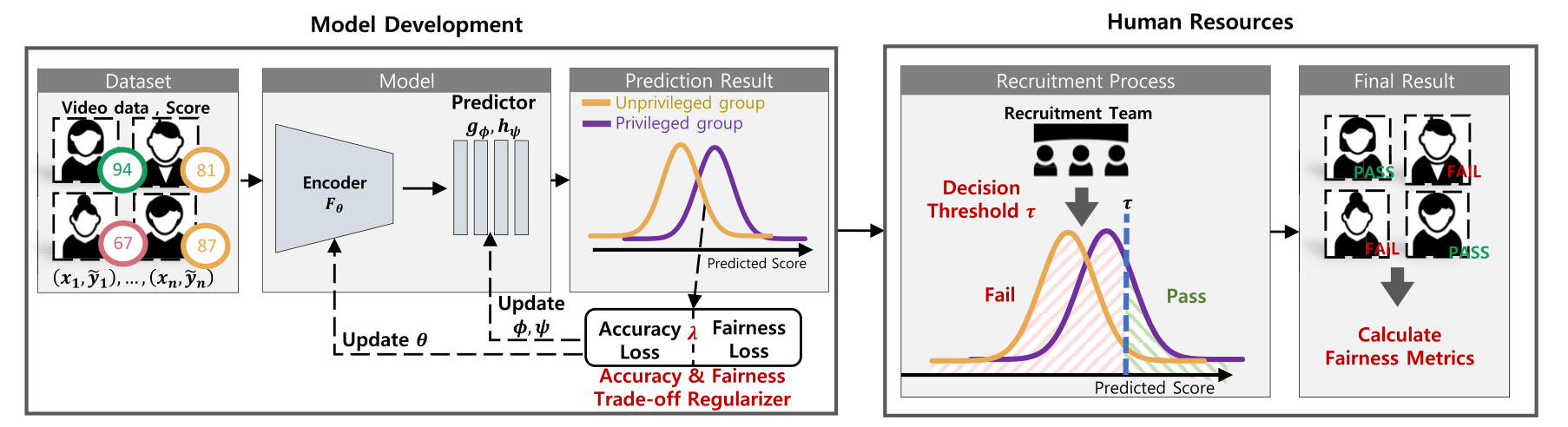
The paper proposes a framework that addresses all three at once. The core ideas are twofold. (1) Reformulate the fairness metric so it does not depend on a single threshold, producing SPDD (Strong Pairwise Demographic Disparity). (2) Exploit the fact that SPDD is mathematically connected to the 1-Wasserstein distance between the two sensitive groups' score distributions, and add the Wasserstein distance itself as a regularizer during training. A single hyperparameter λ_W controls the trade-off between accuracy and fairness.
Method
A Threshold-Free Fairness Metric: SPDD
The most widely used fairness metric, Demographic Parity (DP), is defined for a fixed threshold:
DP(g_τ) = |Pr(Ŷ=1 | S=1) − Pr(Ŷ=1 | S=0)|
S is the sensitive attribute (gender in the paper's experiments); g_τ is the binary classifier built by applying threshold τ. Change τ and DP changes too. When the threshold is set only at deployment time, a single τ-dependent metric is not enough.
The authors define SPDD as the expected DP over τ sampled uniformly from [0, 1]:
SPDD(η) = E_τ~U([0,1]) [ ΔDP(g_τ) ]
If the average DP gap across thresholds is small, the model is fair regardless of the threshold the operator picks.
Connection to Wasserstein Distance
The key insight is that SPDD equals the 1-Wasserstein distance between the per-group score distributions (paper Eqs. 10–11).
Intuitively, the 1-Wasserstein distance is the minimum "amount of work" needed to reshape one distribution into another — picture two piles of earth and the minimum mass-times-distance you would need to move to make one look like the other. Aligning the score distributions of the two sensitive groups in this metric means that, whatever threshold the operator chooses, the pass-rate gap between the two groups stays small.
So minimizing 1-Wasserstein distance is the same as minimizing SPDD. Plug this distance into the loss as a regularizer, and the model aligns the two groups' score distributions on its own during training.
Multimodal Encoder and Adversarial Learning
Video, audio, and text each pass through their own encoder before merging into a shared representation. Video uses a 2D CNN followed by an LSTM; audio runs an LSTM over MFCC features; text uses a pre-trained BERT with a fully connected head. The three representations are concatenated into a common latent space Z.
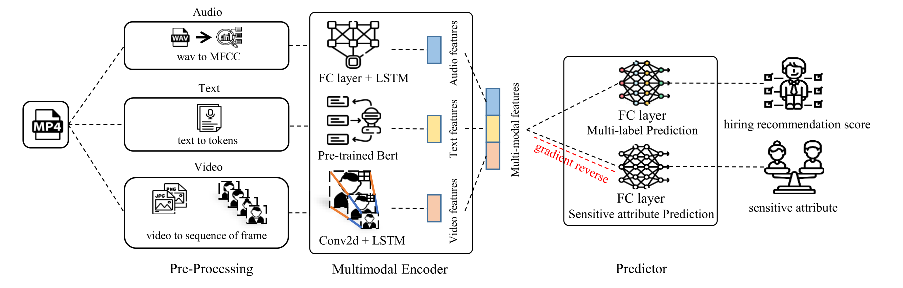
Two heads sit on Z. The regressor gφ predicts the score Ŷ. The adversary hψ predicts the sensitive attribute S. The encoder is trained against the adversary through a gradient reversal layer[6] — that is, the encoder is rewarded for making the sensitive attribute hard to predict from Z.
The Total Loss
The two mechanisms are tied into a single objective:
L_Reg(X, Ỹ) = E[ ‖g(F(X)) − Ỹ‖² ] + λ_W · L_W
L_Adv(X, S) = D_{θ,ψ}(X, S)

min_{φ,ψ} L_Reg(X, Ỹ) + L_Adv(X, S)
min_θ    L_Reg(X, Ỹ) − L_Adv(X, S)
The MSE term carries score-prediction accuracy. The λ_W · L_W term carries fairness through the Wasserstein regularizer. The last two lines spell out the min-max update for the encoder, regressor, and adversary. Larger λ_W tightens fairness; smaller λ_W frees up accuracy.
Why use both mechanisms? The Wasserstein term aligns predicted score distributions, but sensitive-attribute information can still linger in the representation Z itself. The adversary attacks Z directly. The two enforce fairness at different layers, so they need to overlap to be meaningful. The representation-space analysis below confirms this.
Results
Datasets and Bias Injection
The paper evaluates on two datasets.
- HR dataset: about 3,000 Korean-language interview videos. Candidates respond to a fixed prompt within 90 seconds, and labels are the averaged hiring-recommendation score from three interview experts with 20+ years of experience[7]. Sensitive attribute: gender.
- FI dataset: First Impressions (CVPR 2017 ChaLearn Challenge). 10,000 English-language YouTube videos. Sensitive attribute: gender.
The crucial experimental knob is deliberately injected bias. The authors define a parameter α that skews the privileged/unprivileged group ratio in the high-score region (and the inverse in the low-score region). α=2 means 67% privileged in the high band, α=3 means 75%, α=4 means 80%.
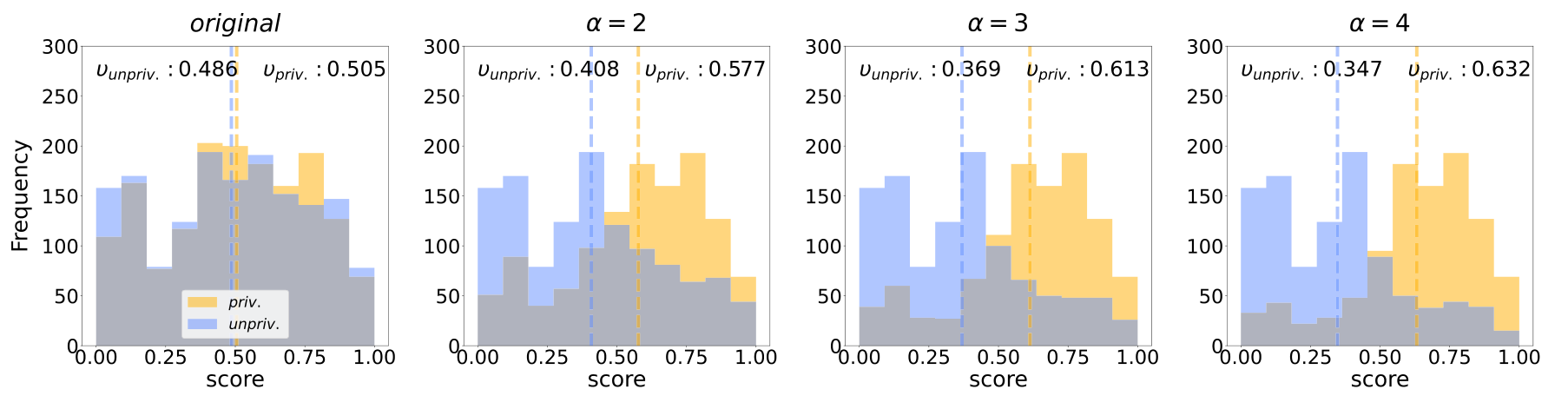
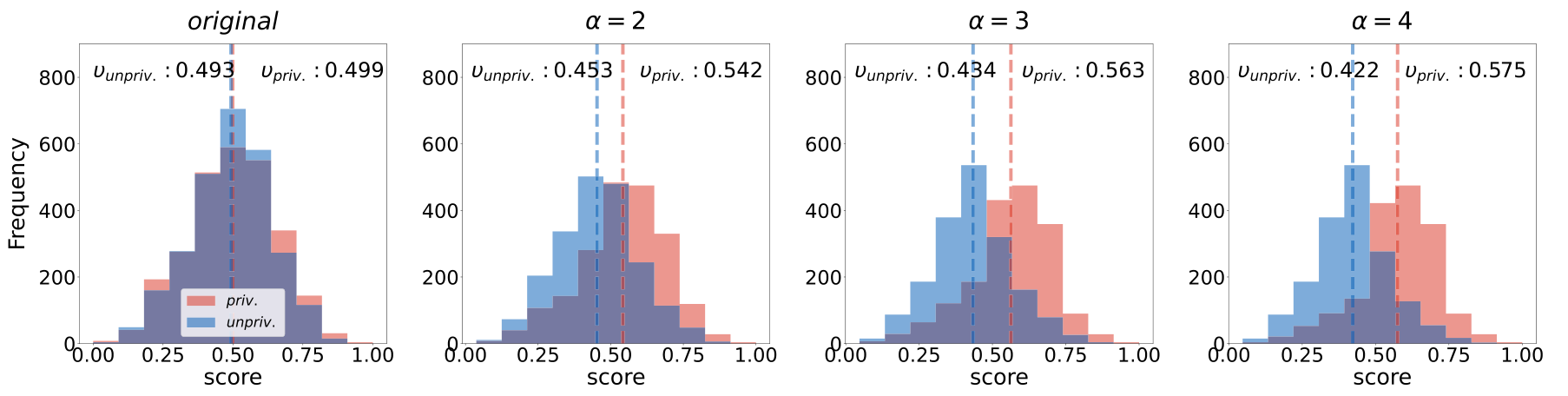
Test sets keep the sensitive attribute balanced, so the experiment can measure how much of the training-data bias gets carried over into predictions.
Quantitative Results
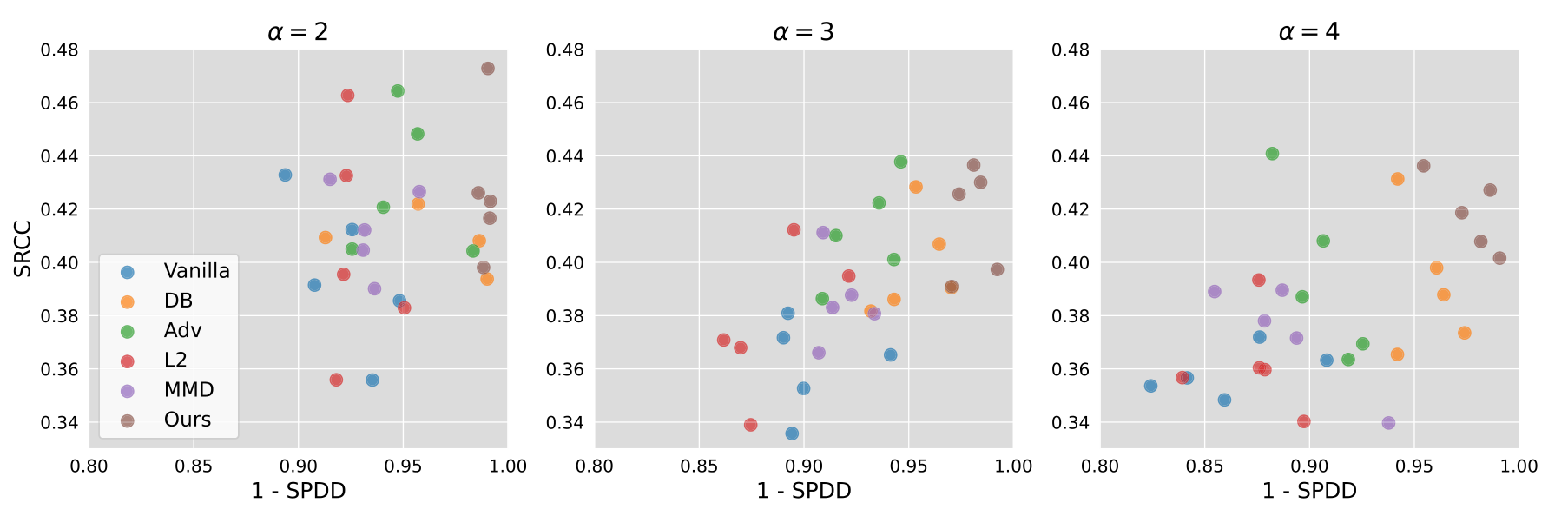
Five baselines are compared: Vanilla (no fairness constraint), Data Balancing (DB), Adversarial training (Adv)[6], Euclidean L2 distance, and MMD (Maximum Mean Discrepancy)[8]. The four evaluation metrics split into two groups — accuracy (PCC, SRCC) and fairness (SPDD, SPEO).
HR dataset at α=4, the harshest bias regime:
| Method | PCC | SRCC | SPDD | SPEO |
|---|---|---|---|---|
| Vanilla | 0.408 | 0.359 | 0.138 | 0.142 |
| DB | 0.434 | 0.391 | 0.043 | 0.041 |
| Adv | 0.433 | 0.394 | 0.094 | 0.098 |
| L2 | 0.407 | 0.362 | 0.127 | 0.129 |
| MMD | 0.420 | 0.374 | 0.110 | 0.104 |
| Ours | 0.458 | 0.418 | 0.020 | 0.016 |
Under the most biased training data (α=4), Vanilla's SPDD is 0.138 while the proposed method drops to 0.020 — roughly a sevenfold reduction. SRCC also climbs from 0.359 to 0.418. The conventional wisdom is that fairness and accuracy trade off, but in this regime the proposed method beats baselines on PCC and SRCC as well as on the fairness metrics. In other regimes and on FI, the fairness lead is even more pronounced while accuracy stays near the top.
The pattern holds at α=2 and α=3 too. The proposed method's HR SPDD stays at 0.011 (α=2) and 0.020 (α=3). On FI at α=4, the method posts SPDD 0.051 vs Vanilla 0.078 and SRCC 0.518 vs Vanilla 0.500.
Fairness in the Representation Space
Beyond the headline metrics, the paper projects the latent representation Z onto a 2-D PCA plane and measures the distance between privileged and unprivileged centroids. Vanilla, Adv, and DB show clear separation. The proposed method produces the smallest centroid distance — meaning sensitive-attribute information is diluted not just at the score level but also in the representation itself.
The Trade-off Curve Through λ_W
Fairness and accuracy can be traded continuously by tuning λ_W.
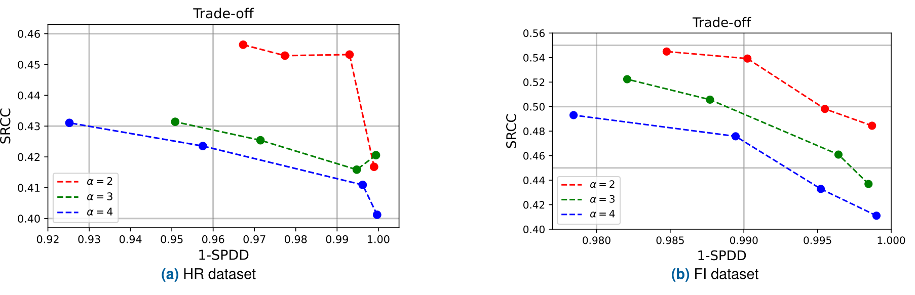
If "how strict should fairness be" depends on domain and operating policy, sweeping λ_W and retraining produces a family of viable operating points — useful in practice.
What It Means for viewinterHR
Genesis Lab's viewinterHR scores video interviews and forwards the scores to hiring teams. The paper's method aligns precisely with the input (video, audio, text) and output (continuous score) structure that viewinterHR handles.
Three points fit directly. First, the threshold τ is set downstream by the hiring team, and the method's fairness guarantee holds across thresholds — a match for real-world operation. Second, extending beyond gender to other sensitive attributes (age, for instance) requires only swapping out the adversary's target. Third, λ_W gives a single knob for setting how much fairness to enforce per domain or per customer policy. Reporting PCC, SRCC, SPDD, SPEO, and the PCA-centroid distance alongside each score turns the fairness claim into something auditable.
The method passed peer review at IEEE Access.
Limitations and Open Questions
The paper itself flags two constraints.
First, sensitive-attribute labels are required during training. In environments with strong privacy regulation (EU GDPR being the obvious case), this premise is hard to satisfy. Achieving fairness without direct use of sensitive attributes is left for future work.
Second, the evaluation covers only asynchronous AVI. Live interviews, game-based assessments, and chatbot interviews shift the data distribution. Whether the Wasserstein-regularizer-plus-adversary scaffolding ports cleanly to those settings is an open question.
The core skeleton, however, holds. Even under continuous scores and multimodal inputs, fairness can be applied directly as a regularization term in the training loss, and a single λ_W moves the accuracy–fairness operating point. That λ_W is best read not as a hyperparameter but as a policy variable — a knob the organization turns to set how strict fairness should be. Fairness in this framing is not a declaration. It is the result of distribution design.
References
[1] Feldman, M.; Friedler, S. A.; Moeller, J.; Scheidegger, C.; Venkatasubramanian, S. Certifying and Removing Disparate Impact. In Proc. 21st ACM SIGKDD Int. Conf. Knowledge Discovery and Data Mining, 2015, pp. 259–268. https://doi.org/10.1145/2783258.2783311
[2] Calders, T.; Verwer, S. Three Naive Bayes Approaches for Discrimination-Free Classification. Data Mining Knowl. Discovery 2010, 21 (2), 277–292. https://doi.org/10.1007/s10618-010-0190-x
[3] Dastin, J. Amazon Scraps Secret AI Recruiting Tool That Showed Bias Against Women. In Ethics of Data and Analytics; Auerbach Publications, 2018; pp. 296–299.
[4] Zafar, M. B.; Valera, I.; Rogriguez, M. G.; Gummadi, K. P. Fairness Constraints: Mechanisms for Fair Classification. In Proc. Artif. Intell. Stat., 2017, pp. 962–970.
[5] Calmon, F.; Wei, D.; Vinzamuri, B.; Ramamurthy, K. N.; Varshney, K. R. Optimized Pre-Processing for Discrimination Prevention. In Proc. Adv. Neural Inf. Process. Syst., 2017.
[6] Ganin, Y. et al. Domain-Adversarial Training of Neural Networks. J. Mach. Learn. Res. 2016, 17 (1), 2030–2096.
[7] Naim, I.; Tanveer, M. I.; Gildea, D.; Hoque, M. E. Automated Prediction and Analysis of Job Interview Performance. In Proc. 11th IEEE Int. Conf. Autom. Face Gesture Recognit. (FG), 2015, Vol. 1, pp. 1–6. https://doi.org/10.1109/FG.2015.7163127
[8] Schumann, C.; Wang, S.; Beutel, A.; Chen, J.; Qian, H.; Chi, E. H. Transfer of Machine Learning Fairness Across Domains. arXiv:1906.09688, 2019.

